Equations

The CL-monodomain problem is a way to approximate the solution of a bidomain problem, with a computational cost that is similar to a monodomain, without assuming the proportionality of conductivity of tensors which leads to the monodomain model.

Solving the CL monodomain consists in first solving a Poisson equation with current boundary conditions on two electrodes, which gives a distribution of electric extracellular potential $\bar{u_\mathrm{e}}$ .

$\left\{\begin{array}{ll} \nabla\cdot((\sigma_\mathrm{i}+\sigma_\mathrm{e})\nabla \bar{u_\mathrm{e}}) = 0 & \mathrm{in}\ \Omega,\\ \partial_n (\sigma_\mathrm{i}+\sigma_\mathrm{e})\bar{u_\mathrm{e}} = I_\mathrm{app}/\left|\Gamma^+\right| & \mathrm{on}\ \Gamma^+,\\ \partial_n (\sigma_\mathrm{i}+\sigma_\mathrm{e})\bar{u_\mathrm{e}} = -I_\mathrm{app}/\left|\Gamma^-\right| & \mathrm{on}\ \Gamma^-,\\ \partial_n (\sigma_\mathrm{i}+\sigma_\mathrm{e})\bar{u_\mathrm{e}} = 0 & \mathrm{elsewhere}.\\ \end{array} \right.$

This problem is ill-posed, so we search the solution with 0 mean value to close the problem. Then, the divergence of the generated electric field is added as source term to the monodomain equation, with a shift in the conductivities used in the operators:

$\left\{\begin{array}{ll} A_\mathrm{m}(C_\mathrm{m} \partial_t v + I_\mathrm{ion}(v,w)) - \dfrac{1}{1+\lambda}\nabla\cdot(\sigma_\mathrm{m}\nabla v) = \nabla\cdot(\sigma_\mathrm{i}\nabla\bar{u_\mathrm{e}}) & \mathrm{on}\ \Omega,\\ \partial_t w + g(v,w) = 0 &\mathrm{on}\ \Omega,\\ \sigma_\mathrm{m}\partial_{\bm{n}} v = 0&\mathrm{on}\ \partial\Omega,\\ + \text{ initial conditions.} \end{array} \right.$

Unknowns

CEPS ID	Name	Math symbol	Unit
0	`Extracellular potential`	$\bar{u_\mathrm{e}}(\bm{x})$	$\si{\milli\volt}$

0	`Transmembrane voltage`	$v(\bm{x},t)$	$\si{\milli\volt}$
-	ionic state variables	$w(\bm{x},t)$	-

Tissue properties

$A_\mathrm{m}$ is the surface to volume ratio of cell membranes, in $\si{\per\centi\metre}$ ,
$C_\mathrm{m}$ is the cell membrane surfacic capacitance, in $\si{\micro\farad\per\centi\metre\squared}$ ,
$\sigma_\mathrm{i}(\bm{x})$ the tensorial intracellular conductivity, in $\si{\milli\siemens\per\centi\metre}$ . Usually, the tensor is the same everywhere when expressed in the local frame defined by fiber orientation. However, alterations of the tissue conductivity can be introduced by using volume fraction.
$\sigma_\mathrm{e}(\bm{x})$ the tensorial extracellular conductivity, in $\si{\milli\siemens\per\centi\metre}$ . Similar to $\sigma_\mathrm{i}$

Other functions

$I_\mathrm{ion}$ is the current due to ionic gates, in $\si{\micro\ampere\per\centi\metre\squared}$ ,
$I_\mathrm{app}(\bm{x},t)$ is the user-defined applied current used to stimulate the domain, through two current boundary conditions corresponding to an anode and a cathode.
is the evolution function of ionic variables.

Usage

Here is an example of input file, which is available in the examples directory. See the input file page for more details on options.

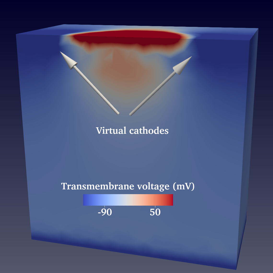
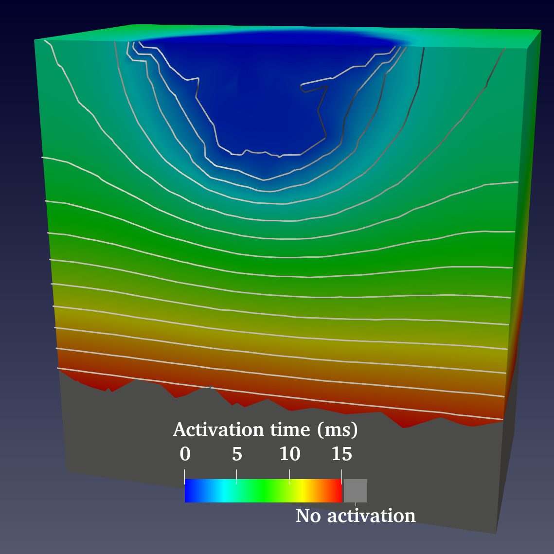
In addition to the usual monodomain results, the generated electric potential is written in separate outputs.

problem type : CLmonodomain
 
#-----------------
# Output controls
 
# Output name
output file name : ./results/CLmonodomain
# Output every 0.5ms
output period : 0.5
 
# Data used to generate the activation time map. Values are
# - Unknown index
# - AP detection threshold (mV)
# - Minimum voltage used for peak detection (mV)
# - AP duration percentage
activation time data : 0 -20 -40 0.75
 
#-----------------
# Simulation time
 
# Times are given in milliseconds
PDE start time : 0.0
PDE end time   : 15
 
#----------
# Geometry
 
# Meshes
3d mesh : ./meshes/clMesh
# to make it [-5,5]
geometry scale : 10 
 
#--------
# Tissue
 
# Surface to volume ratio, in cm-1
Am : CONSTANT 2.0
 
# Conductivity, in mS per cm
intracellular conductivity : CONSTANT 3.6 0. 0. 0. 0.8 0. 0. 0. 0.8
extracellular conductivity : CONSTANT 3.6 0. 0. 0. 1.2 0. 0. 0. 1.2
 
#-------------
# Ionic model
 
# Format: unknownIndex ionicModelName <regionAttributes>
ionic model : 0 MS
 
 
#-------------
# Stimulation
 
# Region attributes of electrodes
anode   attributes : 10 
cathode attributes : 20
 
# A time function can be used to describe the intensity of the current 
# delivered by the electrodes
electrodes stimulation : TIME PROFILE CONSTANT START 0.04 DURATION 1. AMPLITUDE -15000.
 
 
#----------------
# solver options
 
# Only FE 1 available for now
spatial discretization : FE 1
# Time scheme for PDE solving
PDE solver             : SBDF 2
PDE time step          : 0.01
 
# Linear solver options
linear solver absolute tolerance : 1.E-12
linear solver relative tolerance : 1.E-12
linear solver type               : GMRES
 
# Ionic solver. Here Rush Larsen of order 2.
ionic model solver : RL 2

There you can already see on this very coarse mesh the effect of the difference in anistoropy ratio between intra and extracellulat conductivities that creates virtual cathodes around the anode.